The Big O Notation is a way to describe the performance or complexity of an algorithm. It is used to evaluate how much time or space an algorithm will require as the size of the input data grows.

How does it work?

The Big O Notation is represented using the letter “O” followed by a function that describes the relationship between the problem size and the amount of resources used. The variable “n” represents the number of operations performed by the algorithm.

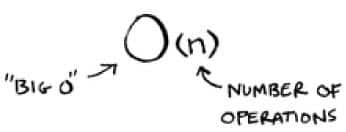
Illustration from the book "grokking algorithms"

For example, O(n) indicates that the algorithm has a linear time complexity, meaning that the function grows proportionally to the problem size.

Types of Big O Notation

• O(1): Indicates that the algorithm has constant time complexity. This means that the execution time does not depend on the problem size. It doesn’t matter if the problem has 10 elements or 10,000 elements, the algorithm will take approximately the same amount of time to execute.

It is considered the ideal case of efficiency since the execution time is constant and unaffected by the problem size.

• O(n): Indicates that the algorithm has linear time complexity. This means that the execution time increases proportionally to the problem size. If the problem size doubles, the execution time will also double.

For example, if you have a list of n elements and you traverse them one by one, the execution time will be proportional to the number of elements in the list. Algorithms with this complexity are commonly found in search operations and linear traversals.

• O(log n): Indicates that the algorithm has logarithmic time complexity. This means that the execution time increases logarithmically as the problem size increases. In other words, as the problem size doubles, the execution time only increases by a constant amount.

This type of complexity is commonly found in binary search algorithms and data structures like balanced trees. Algorithms with logarithmic complexity are considered very efficient.

• O(n^2): Indicates that the algorithm has quadratic time complexity. This means that the execution time increases quadratically with the problem size. If the problem size doubles, the execution time will increase by approximately four times. Algorithms involving nested loops often have this complexity.

It is important to be cautious with this complexity, as it can lead to significant execution time for large problem sizes.

• O(2^n): Indicates that the algorithm has exponential time complexity. This means that the execution time increases rapidly as the problem size grows. For each additional element in the problem, the execution time doubles.

Algorithms with this complexity are considered inefficient and can become impractical for moderately large problem sizes. More efficient alternatives should be sought when dealing with algorithms of this complexity.

• O(n!): Indicates that the algorithm has factorial time complexity. This means that the execution time grows factorially with the problem size.

Factorial complexity is the worst of all, as it implies that the execution time grows exponentially with each additional element. Algorithms with this complexity are extremely inefficient and generally not viable for moderate or large problem sizes. Alternative approaches or more efficient algorithms should be sought to solve this type of problem.

• O(n log n): Indicates that the algorithm has a time complexity of n log n. This means that the execution time increases proportionally to the product of the problem size and the logarithm of the problem size.

This complexity is commonly found in efficient sorting algorithms like Quicksort and Merge Sort. Although it is more efficient than quadratic complexity (O(n^2)), it is still less efficient than linear complexity (O(n)) or logarithmic complexity (O(log n)). Algorithms with this complexity are used for sorting or performing operations on moderately to large-sized data sets.

Let’s take a look at a graph to see how these types of notations are represented!

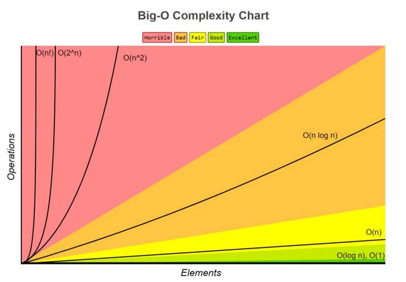
Graph from the book "grokking algorithms"

In this graph, we can observe that algorithms located in the red zone are the least efficient. In the orange zone, although they improve compared to the red zone, they are still considered less efficient. Algorithms in the yellow zone show normal efficiency, while those in the light green zone are considered more efficient. Finally, the best algorithms are found in the green zone.

Conclusions

In conclusion, the Big O Notation is a fundamental tool for describing the complexity and performance of algorithms. Through this notation, we can evaluate how the execution time or resource usage varies as the problem size grows.